Developing an app to interpret chest X-rays to support the diagnosis of respiratory pathology with artificial intelligence

Introduction

Medical images, including results from X-rays, are an integral part of medical diagnosis. Their interpretation requires an experienced radiologist, a human whose skills are scarce and who can commit mistakes when tired. But at face value, the X-ray diagnostic uses simple features from the image, such as black and white intensity, contours and shapes, all properties which an artificial intelligence (AI) can handle well.

And indeed, in recent years, the idea of using AI as a means of assisting diagnostic (classification) has taken hold, thanks to the increase of computational speed (e.g., with graphical processing units, a.k.a. GPUs), the availability of large and well-documented data sets, and the development of deep learning techniques, in particular convolutional neural networks (CNNs). The results of a number of studies training CNNs to diagnose diseases using 2D and 3D images are rather impressive, reaching near 100% accuracy in such diverse pathologies as lung nodules or Alzheimer’s, see Ref. (1) for a recent overview. Moreover, in some cases the performance of the AI exceeds that of radiologists, see, e.g., the study of CheXNet (2).

One of the main problems faced by people in developing countries is access to timely medical diagnosis. Lack of investment in health care infrastructure, geographical isolation and shortage of trained specialists are common obstacles to providing adequate health care in many areas of the world.

Yet the use of AI is still limited for various reasons, technical and sociological. For example, images are only one aspect of the patient history which can be supplemented with clinical signs, e.g., whether the patient has fever. Currently, the availability of databases with additional clinical information is scarce, but databases with better labelling could substantially improve the AI training in the near future. A more important issue is related to the natural variability of a large training data set, and the need to remove modelling when interpreting the image. This has led to the development of new techniques beyond CNNs (supervised learning) to incorporate a more bottom-up approach: unsupervised machine learning. Nevertheless, all these studies rely on a large number of neuron layers, typically dozens, and good quality images. The trained neural network (NN) can then be used in a powerful computer station to help diagnosis.

Given our interest in portability, we need to develop a different strategy. We cannot deploy machine learning algorithms which depend on too many layers, and we cannot rely on the acquisition of precise images. Instead, we have to strike a balance between the desired outcomes (portability and reliability) and the real-life situations a clinician may encounter on field.

This note presents our results to help the early diagnosis of a number of life-threatening conditions in remote areas with the use of new methodologies (based on Machine Learning) and their capability to be deployed into mobile devices. We use the latest developments in AI environments which are portable and fast, in particular Fast.AI (3), to develop an artificial NN to be deployed as a smartphone app, or in one of Google’s AI development kits, or in Raspberry PI, as a tool to assist physicians in their diagnostic. A beta version of the app can be tested in the Heroku environment (4) and all the code developed during this project can be obtained in GitHub (5).

Methods

The data set and analysis framework

We use the ChestX-ray14 data set (6) which contains 112,120 frontal-view X-ray images of 30,805 unique patients. The images are frontal view of chest X-rays PNG images in 1,024×1,024 resolution. Meta-data for all images contains: image index, finding labels, patient ID, patient age, patient gender, view position, original image size and original image pixel spacing. Each image contains the annotations up to 14 different thoracic pathology labels. The labels were assigned using automatic extraction methods on radiology reports. The database from NIH is available on-line through the link: https://nihcc.app.box.com/v/ChestXray-NIHCC/folder/36938765345.

The 14 common thorax disease categories are: atelectasis, cardiomegaly, effusion, infiltration, mass, nodule, pneumonia, pneumothorax, consolidation, oedema, emphysema, fibrosis, pleural thickening, and hernia.

Regarding the analysis of the dataset, in this project we use AI techniques in the framework of Fast.AI (3), a library which simplifies accurate and fast training of NNs using modern best practices. It includes out-of-the-box support for vision, text, tabular, and collaborative filtering models. Another main advantage of Fast.AI is the simplification of the data processing made by the data block application programming interface (API), and the implementation of the fit one cycle method (7) and mixed precision training (8). The fit one cycle method allows us to drastically reduce the training time by allowing changes during the training in the learning rates and momentum (hyper-parameters). This method can reduce the time to train big NN models, but also stabilize it by helping the optimization algorithm to prevent falling into saddle points. The mixed precision training uses half-precision floating point numbers, without losing model accuracy or having to modify hyper-parameters. This nearly halves memory requirements and, on recent GPUs, speeds up arithmetic calculations.

Selecting and processing the data

Since we are interested in distinguishing different types of diseases, we will focus on the dataset with labels of at least one disease. In the data set there are 51,759 images with at least one disease (non-healthy). On this data set, we will perform two types of analyses: (I) one vs. all and (II) multi-label classification.

In the first type of analysis, we will train an algorithm to identify patients with a specific disease, which we choose to be Pneumothorax for illustrative purposes, versus any other type of disease in the sample. In the second type of analysis, we will tackle a more difficult but realistic situation: often diseases do not occur in isolation, e.g., atelectasis tends to appear in conjunction with cardiomegaly or consolidation, or both. This more complex situation is called co-occurrence, which in terms of the data analysis corresponds to a problem of multi-label classification.

Below we describe how we select and process the data in these two situations:

One vs. all problem (i.e., pneumothorax vs. all)

We separate the data set in two categories, one with the label pneumothorax the other with all the images with no pneumothorax label (atelectasis, pneumonia, ...). Specifically, we first read from the metadata information available in the file Data_Entry_2017.csv the images names and findings, selecting the entries with the pneumothorax label to one folder and all the others to a different folder. After this selection one ends up with the following set of samples:

• Pneumothorax: 5,302 images, resolution 1,024×1,024 8-bit gray scale;
• No-pneumothorax: 46,457 images, resolution 1,024×1,024 8-bit gray scale.

Next, we prepare the data for testing and validation using the Fast.AI data block API, which automatically loads the data from their respective folders, assign their labels according to the name of the folders and split the full data into training (80%) and validation (20%) data sets. The data block API ensure the use of correct labels, the correct train/validation (or test) split, the correct normalization of the images and all the augmentations transformation we later apply¹. After this selection and transformations, we end up with:

• Train size (80%): 41,408 items, items dimension: 224×224 three channels, transformation applied;
• Validation size (20%): 10,351 items, items dimension: 224×224 three channels, no transformations;
• Batches which are set to 64 items per batch, so they can fit on a regular GPU memory.

We select the following transformations to be applied to the train data set:

• Random rotation (clockwise or counter-clockwise) in an angle range between 0 and 30 degrees;
• Fifty percent chance of an image to be zoomed by a 1.3 scale;
• One hundred percent chance of an image be selected to randomly modify brightness and contrast within a range between 0 and 0.4;
• Normalize the items according to the stats of each batch, i.e., take the mean and the standard deviation of each channel and normalize the image using them².

Note that the images fed into the CNN are set to be 224×224 with three channels due to hardware limitations and the size of the batch (64 images) to fit into the GPU memory, as well as coding implementation—the CNN architecture we are using (DenseNet) was originally designed to work with three channels (RGB), so the input layer is designed to take inputs (tensors) with the dimension (batch size, C =3, x size, y size) where C is the number of channels from the image.

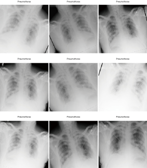
In Figure 1 we show the effects of the transformations we apply in the train data set items. They are designed to emulate some of the issues which different situations could lead to. For example, brightness variance can occur when the technician exposes the patient to a more energetic X-ray beam (higher keV X-rays) or long exposure time, which greatly increases the contrast of the image, but also increases the radiation dose received by the patient; or in the case of film X-ray, the exposure time to chemicals can drastically reduce contrast of the image, leading to erroneous feature differentiation.

Figure 1 Random transformations applied in one selected image. The random rotation and change in brightness are applied to consider the variations of image quality and arrangement one can encounter in medical facilities in remote areas.

Multi-label classification

For the multi-label case we prepare a new csv file which contains the name of the image (in our input data set the names are formatted as 00025252_045.png) and the label of the diseases found in the respective images. This file will be used by the data block API to correctly label the images. The file Data_Entry_2017.csv contains all the metadata with the name of each image together with the findings and other information that can be used for future applications.

To create the multi-class label file we use a python script with two main functions: one to extract the information from the Data_Entry_2017.csv metadata and another function to write the new csv file with the columns contain the path to the images, their respective findings and a new column with a one-hot encode³ to represent the presence or not of each disease (class) in a given image, in Figure 2 we show the structure of the Data_Entry_2017.csv.

Figure 2 Extract of the label data frame for the multi-label classification task. Fast.AI can handle multi-label classification targets and image names are given in a proper structured way, which we provide a new csv file. The one-hot encode represents the presence [1] or absence [0] of a particular disease in the list: atelectasis, cardiomegaly, effusion, infiltration, mass, nodule, pneumonia, pneumothorax, consolidation, edema, emphysema, fibrosis, pleural thickening and hernia.

The Fast.AI API contains a very convenient method to prepare and load the images into our CNN model called ImageDataBunch, which contains a series of useful functions which one can use for AI purposes. For example, for the multi-label classification one can use the ImageDataBunch.from_csv(), which automatically identifies the images and multi-class labels we are loading into the CNN, e.g., np.random.seed (42).

data = ImageDataBunch.from_csv(path, label_delim=’|’, csv_labels=’label list.csv’, label_col=1,\ delimiter=’,’, valid_pct=0.2,ds_tfms=tfms,bs=64, size=224,num_workers=3).normalize()

This set of commands will automatically load the images in batches of 64, re-size the images form 1,024×1,024 to 224×224, load the labels from labellist.csv and normalise according to the pytorch standard, and split the dataset into 80% test images and 20% for validation.

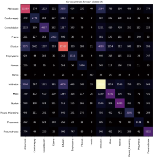
A very important aspect in our analysis is how often one disease appears together with others, i.e., the rate of co-occurrences. We can check the co-occurrences of a disease using scikit-learning feature extraction library, and in Figure 3 we show the matrix of number of co-occurrences in the data set. This information is key to introduce the proper weights used in the loss function and lead to the positive identification of a given class. These values can help us to better calibrate the weights for each class in order to avoid situations like a model who can only predict the class where one has the higher number of targets.

Figure 3 Number of co-occurrences for each disease in the data set. Note, for example, that Infiltration is always co-occurrent with some other disease label, and that some diseases often come together, e.g., effusion and atelectasis.

The model architecture and training

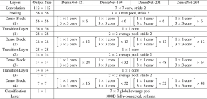
Our architecture will be based on the DenseNet-121 model with the last layers (header) modified for our purposes. Specifically, our CNN model consists on the following parts:

• The body of the model is the same as the DenseNet-121, described in Figure 4 (third column) (DenseNet-121);
  

  Figure 4 DenseNet architectures for ImageNet. Note that each “conv” layer shown in the table corresponds the sequence: batch normalization, rectifier linear function and a convolutional layer (BN-ReLU-Conv).
• For the classification layer, we remove the last layer from DenseNet-121 and replace it with the following layers:
  • AdaptiveConcatPool2d layer;
  • Flatten layer;
  • A block with [nn.BatchNorm1d, nn.Dropout, nn.Linear, nn.ReLU] layers.

In our loss function we use the weights from each class calculated according to the scikit-learn class weight method, defined as:

nsamples(nclasses∗[n1,n2,…])[1]

Where n_samples is the total number of images in the training sample, n_classes is the number of classes (2 in the case of one vs. all), and n₁, n₂, … are the number of images for each class. This function from sklearn returns the weight for each class in our training sample, information we pass onto the weights in the loss function, which mitigates the problem of having more images from one class than another class, i.e., imbalanced classes data sets.

The network is trained end-to-end using Adam as an optimizer (9) with standard parameters (β₁ =0.9 and β₁ =0.999). We trained the model using the fit one cycle method (7), which consist in the following steps: initializes the training with a given learning rate and momentum; in the middle of the training phase the learning rate is increased up to a given maximum value while the momentum is reduced; and close to the end of the training the learning rate is reduced again and the momentum increased, as shown in Figure 5. This method gives more stable results by avoiding the optimization process to fall into saddle points and requires less epochs to fully train our model.

Figure 5 Fit one cycle method. Left figure: this shows the variation of the learning rate over the number of iterations, with the vertical axis showing the learning rate change between 1e⁻⁴ to 3e⁻³ and the horizontal axis showing all the iterations (i.e., epochs). Right figure: here we show the change in momentum rate over number of iterations. In these figures we can see the change in values of the learning rate and momentum, during the middle of the cycle. The high learning rates and small momentum will act as regularization method, and keep the network from overfitting, as they prevent the model from landing in a steep area of the loss function, preferring to find a minimum that is flatter.

Another useful parameter for training our CNN is the weight decays⁴. After each epoch, the weights of the NN are multiplied by a smaller factor between 0 and 1. This is one of the various forms of regularization of the NN training, together with batch size and dropout (10). One can choose a weight decay which allows us to use a bigger initial value for the learning rate and thus reduce the time of training during the fit one cycle.

For the one-vs-all case we choose the Cross Entropy Loss with weights defined for each class to take into account the high imbalance between the pneumothorax case vs. all the others. Specifically, to apply the weights into our loss function we do as follows:

class_weights = torch.FloatTensor(weights).cuda() loss_func = nn.CrossEntropyLoss(weight=class_weights)

where the weights are calculated by the Equation [1], the function cuda() just moves the numbers calculated for the weights to the GPU memory where our CNN is loaded. The weights are passed to the loss function by the argument weight from the cross entropy loss class.

The Cross Entropy Loss function, in the case of the class weight argument being specified, can be described as:

loss(x,class)=weight[class](−x[class]+log(∑jexp(x[j])j))[2]

with x as the image input for the respective class.

Another important aspect for the Cross Entropy Loss is the reduction method, which specifies the reduction to apply to the output. The pytorch framework gives three options: none, mean and sum, we choose mean in our analysis. For the multi-label classification task we choose BCEWithLogitsLoss. This loss combines a Sigmoid layer and the BCELoss in one single layer. By combining the operations into one layer, one takes advantage of the log-sum-exp trick (11) for numerical stability.

The BCEWithLogitsLoss for the multi-label case with class weights is described by:

lc(x,y)=Lc={l1,c,…,lN,c}Τln,c=−wn,c[pcyn,c⋅logσ(xn,c)+(1−yn,c)⋅log(1−σ(xn,c))][3]

where c is the class number (c >1 for multi-label binary classification, c =1 for single label binary classification), n is the number of the sample in the batch and p_c is the weight of the positive answer for the class c. Note that p_c >1 increases the recall, whereas the choices with p_c <1 increase the precision. Also note that we used the default option mean as reduction method to BCEWithLogitsLoss.

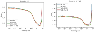
Before training, one has to define the range of the learning rate to be used in the fit one cycle method. To compute the best range for the learning rate we used the function learner.lr_find(), which will perform a test run, starting with a very small learning rate and increasing it after each mini-batch until the loss function starts exploding. Once the loss starts diverging, the lr_find()will stop the range test run. In Figure 6 we show the loss values vs. the learning rate for each weight decay choice (WD =0, 0.1, 0.001, 1e⁻⁵). The best initial values for learning rates are the ones giving the steeper gradient towards the minimum loss value (7). In the case of Figure 6 this value is 1.32e⁻² for the left figure and 1.02e⁻² for the right one.

Figure 6 Effect of the different choices for the weight decay (WD) in the loss change (vertical axis) for a given learning rate (horizontal axis) for the DenseNet-121 CNN without class weights (left panel) and with class weights (right panel). Note that the loss is relatively insensitive to the choice of WD, which is a sign of stability of our model. With small values for the WD one can choose large values for the learning rate and reduce the training time (i.e., number of epochs). CNN, convolutional neural network.

The learning rate change can be described as follows:

n=number of iterations

max_lr=maximum learning rate

init_lr=lower learning rate (we start the range test from this value)

max_lr=init_lr * qⁿ

q=(max_lr/init_lr)1n[4]

Note that the learning rate after the i-th mini-batch is given by:

lri=init_lr∗(max_lr/init_lr)in[5]

We are using the transfer learning methodology to not just training our CNN faster, but also to increase the accuracy. To execute this task, we trained the CNN in two phases. During the first phase, the model is trained from end-to-end, i.e., all the layers are trained, for 30 epochs with an initial learning rate of 1.32e⁻² to a maximum 1e⁻¹. This initial value is chosen due to the loss value for this learning rate exhibit the steeper gradient value towards the direction of the minimum, as we can see in Figure 6. After the 30 epochs, the training is stopped and the weights are saved, leading to a second train phase which uses the weights saved from the previous training, freeze all the layers before the last classification layer to void retraining all the NN, and train only the last classification layers with a different range for the learning rate. This process described above is what we know as transfer learning, and we evaluate the impact of this methodology on the accuracy of our model between the two phases.

Results

In a simple binary classification problem (like in our benchmark pneumothorax vs. all), one can define some measures of how well our algorithm is performing: precision, accuracy and recall. All these are computed by evaluating how often in a sample the results lead to a true-positive (TP), true-negative (TN), false-positive (FP) and false-negative (FP) diagnoses. Based on these numbers one can define three measures of goodness of diagnosis:

Accuracy = TP + TN/TP + FP+ FN + TN, the ratio of correct observations vs. all observations, e.g., accuracy would tell us how likely is to correctly identify pneumothorax pathologies in sick patients.

Precision = TP/TP+FP, the ratio of correct predicted positives vs. all the classified as positive, e.g., precision would tell us how many patients diagnosed with pneumothorax do actually have pneumothorax.

Recall (or sensitivity) = TP/TP+FN, the ratio of correctly predicted positive vs. all the elements with the actual disease, e.g., recall would tell us the probability for correctly diagnosing pneumothorax among all the patients suffering from pneumothorax.

Obviously, all these measures are important, and depending on the nature of the disease and focus of the practitioner the algorithm could be trained to improve any of these three, usually at the cost of the other two. A typical average measure of goodness which works well in imbalanced data sets is the F1 score, defined in its simplest form as an average between accuracy and recall

F1 score = 2 * (precision * recall)/(precision + recall)

Results for one vs. all (pneumothorax)

We can compute the F1 scores and precision-recall (PR) of our CNN using our validation data set. In scikit-learn, F1 scores can be evaluated using different average methods⁵, namely:

• Binary: only reports results for the class specified by positive label, i.e., Pneumothorax detected. This method is only applicable in the binary problem (pneumothorax vs. all) but not in the multi-class problem;
• Micro: this method counts the total true positives, false negatives and false positives, to compute a more global metric;
• Macro: in this case, the function calculates the metrics for each label and find their unweighted mean, i.e., it does not take label imbalance into account;
• Weighted: in this case, the function finds metrics for each label, and their average weighted by the number of true instances for each label. This is an improvement from “macro” to account for label imbalance.
• Samples: In this case, the function calculates metrics for each instance, and find their average. This is only meaningful for multi-label cases.

Since we are dealing with high imbalanced classes, we will be using the weights for our samples from the validation data set:

W_validation = [All others: 0.5566, Pneumothorax: 4.902][6]

With these weights we can build an array with the same size as the ground labels and evaluate all the metrics taking into account the class imbalance. The results are as follows:

• F1 score (macro): 0.5822911828419564;
• F1 score (micro): 0.6762802817903739;
• F1 score (weighted): 0.7132615220206845;
• F1 score (binary): 0.384149629028795;
• F1 score (All others, Pneumothorax): [0.7804330.38415].

And show the range of different F1 scores one can obtain, even in the binary classification problem.

There are two common representations of the goodness of the algorithm. One is the PR curve, shown in Figure 7. A high area under the curve represents both high recall and high precision and is an indication of good performance.

Figure 7 Precision-recall (top) and ROC (bottom) curves for our model in the pneumothorax vs. all case. ROC, receiving operating characteristic.

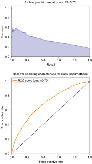
Another representation is the so-called receiving operating characteristic (ROC) curve which shows the shape of TP as a function of FP. One often says that the algorithm learns when the curve is steeper than a straight line, namely the algorithm is doing better than a 50% chance of identifying the right disease (better than a random pick). In Figure 7, the orange line corresponds to the ROC curve of our algorithm, which is clearly performing better than chance. A related and more global measure of goodness based on the ROC plot is the area under the curve (AUC), and in this figure AUC is 70% for detecting pneumothorax.

Layers heatmaps

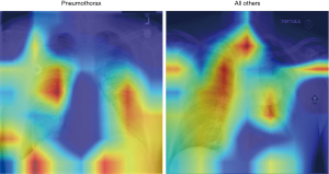
To visually understand what regions in the image our CNN is picking up on, we look at the area of the image which is more active when we show an image from a given class. To do this, we built a Grad-CAM following Ref. (12).

In Figure 8, the regions displayed in yellow to red colour highlight the spatial location of the features which activate more intensely the last convolutional layer before the classification. As one can see, in the pneumothorax image the CNN is identifying important features located in the left lung, top of diaphragm and a region below the right lung. Meanwhile, for the non-pneumothorax image the CNN identify as hot regions on the top of diaphragm, apex of the heart and a hot spot on the left side outside of the body. These images provide valuable information about what are the most important features for our CNN and how to tune the parameters of the model to improve the training phase. One conclusion we can extract from these images is that, although overall, we are getting good classification scores, the CNN is struggling to localize good features to better classify the images. We plan to use this method to improve on the training, by including more random transformation like flip horizontal and vertical, random crop and a different pad method.

Figure 8 Grad-CAM for a pneumothorax item (left) and no Pneumothorax item (right) class. The regions in red show the areas which activate more units (neurons) in the last convolutional layer before the classification.

Results for multi-label

We move onto a much more complex case, where instead of a binary classification problem pneumothorax vs. no-pneumothorax, we tackle the classification of 14 diseases, including the additional difficulty of co-occurrence of various diseases in the same patient.

The first thing we need to do is to define new measures of goodness for our method. PR or ROC curves like Figure 7 are designed to understand a binary classification problem.

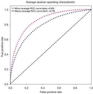
We need to generalize these two notions to a multi-classification case. For example, one ROC curve can be drawn per label, but one can also draw a ROC curve by considering each element of the label indicator matrix as a binary prediction (micro-averaging). Another evaluation measure for multi-label classification is macro-averaging, which gives equal weight to the classification of each label.

The “micro-average”, purple dashed curve Figure 9, is calculated as each element of the label indicator matrix, in our case a matrix with the dimensions (number of validations samples, number of classes), as a binary prediction. For the “macro-average” we first need to aggregate all elements from the false positive rate (fpr) of each class and casting them into a list which we call all_fpr. From this list we can interpolate each aggregated fpr and the ROC curves of each class we have calculated. By averaging the interpolated points computed previously over the number of classes (14 for our data), we obtain the mean of the true positive rate for all classes (blue dashed curve, Figure 9).

Figure 9 Micro and macro ROC average for multi-label class. For the micro-average we got AUC =82%, while for macro-average we obtain AUC =72%. ROC, receiving operating characteristic; AUC, area under the curve.

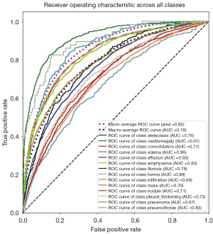
We can also compute the ROC and AUC for each class using the predictions and the truth information for each class. The results are shown in Figure 10, where we display all ROC and AUC for the 14 classes including the micro-average and macro-average.

Figure 10 ROC curve for each of 14 classes and their respective AUC. The higher AUC we get is for cardiomegaly AUC =85%, while the lowest we get is for mass (AUC =56%), pneumothorax we got AUC =74%. ROC, receiving operating characteristic; AUC, area under the curve.

As discussed in the previous section (pneumothorax vs. all), the PR plot is a useful measure of prediction success when the classes are very imbalanced. In Figures 11,12, we show the PR curves for the average and for each class, respectively.

Figure 11 Precision-recall curve considering micro-average, i.e., an aggregate of the contributions from each class and average over all classes. In a multi-class classification, micro-average is preferable to macro-average for class imbalance. AP, average precision.

Figure 12 Precision-recall curves for each of the 14 classes and their respective areas. The areas are calculated using the average precision score considering the weights of each class. The iso-curves show the F1 scores in the precision-recall plane.

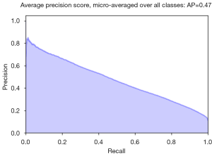
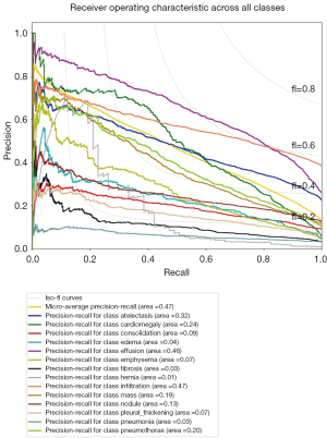
The average precision (AP) summarizes the PR plots as the weighted mean of precision achieved at each threshold, with the increase in recall from the previous threshold used as the weight:

AP=∑n(Rn−Rn−1)Pn[7]

Where R_n and P_n are the precision and recall at the n-th threshold.

Finally, in Tables 1,2 we quote the values of the AUC score and the AP for each class.

Layers activation maps and Guided-Grad-CAM

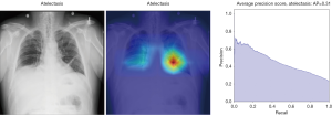
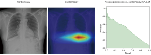
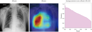
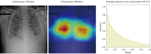
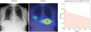
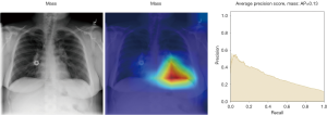
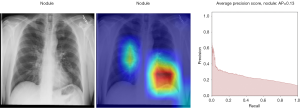
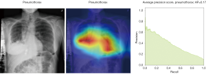
Here we perform a similar study as in the pneumothorax vs. all case by identifying the regions in the image which activates neurons in the CNN. All the images used in to generate the activation and Grad-CAM maps are from the validation data set, namely these are images the CNN never saw before. In the next Figures 13-20, we show examples for different pathologies: the input figure, the Grad-CAM heatmap, and the PR curve related to the specific class.

Figure 13 Original image (left), Guided Grad-CAM (center) and precision-recall (PR) plot (right) for Atelectasis class. The Grad-CAM shows that the CNN is getting very hot spots (regions in red) in the left lung and at the bottom of the right lung. The PR curve for this class gives AP =0.31. CNN, convolutional neural network; AP, average precision.

Figure 14 Original image (left), Guided Grad-CAM (center) and precision-recall (PR) plot (right) for cardiomegaly class. The Grad-CAM shows that the CNN is getting a very hot spot in the bottom left region. The PR curve for this class gives AP =0.21. CNN, convolutional neural network; AP, average precision.

Figure 15 Original image (left), guided Grad-CAM (center) and precision-recall (PR) plot (right) for effusion class. The Grad-CAM shows that the CNN is getting a very hot at the right lung. The PR curve for this class AP =0.42. CNN, convolutional neural network; AP, average precision.

Figure 16 Original image (left), guided Grad-CAM (center) and precision-recall (PR) plot (right) for emphysema class. The Grad-CAM shows that the CNN is getting hot spots at the both lungs. The PR curve for this class gives AP =0.07. CNN, convolutional neural network; AP, average precision.

Figure 17 Original image (left), guided Grad-CAM (center) and precision-recall (PR) plot (right) for Infiltration class. The Grad-CAM shows that the CNN is getting a very hot region on both lungs, same as the Hernia case. The PR curve for this class gives AP =0.46. CNN, convolutional neural network; AP, average precision.

Figure 18 Original image (left), guided Grad-CAM (center) and precision-recall (PR) plot (right) for mass class. The Grad-CAM shows that the CNN is getting very hot region on the left lungs. The PR curve for this class gives AP =0.13. CNN, convolutional neural network; AP, average precision.

Figure 19 Original image (left), guided Grad-CAM (center) and precision-recall (PR) plot (right) for nodule class. The Grad-CAM shows that the CNN is getting a hot region on left and right lungs. The PR curve for this class gives AP =0.13. CNN, convolutional neural network; AP, average precision.

Figure 20 Original image (left), guided Grad-CAM (center) and precision-recall (PR) plot (right) for pneumothorax class. The Grad-CAM shows that the CNN is getting a hot region on both lungs. The PR curve for this class gives AP =0.17. CNN, convolutional neural network; AP, average precision.

Weighted vs. unweighted (ROC vs. PR) for multi-label classification

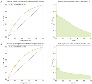
We noticed that for multi-label classification CheXnet use unweighted binary cross entropy losses. This might not be problematic since in their paper the authors compare the AUC from the ROC metrics with the state of the art models for the ChestX-ray14 data set. ROC curves have an attractive property: they are insensitive to changes in class distribution. If the proportion of positive and negative classes changes in a test set, the ROC curves will not change. To compare with our results we first implemented our loss function without considering the weights for each class. The results are displayed in the Figures 10-12 as well in Table 1. However, due to the class imbalance the PR curves tell us a very different history from the ROC curves.

Indeed, by comparing Figure 21, we see that while the ROC curve for unweighted loss seems to indicate a very good classification, one should consider that reality is different: we are dealing with a very skewed class distribution, e.g., some labels have samples with order 10⁴ inputs (atelectasis) while others only a few hundred samples (Hernia). In this situation, the ROC does not tell the full history of our classification model. We have to also consider cases where we have few samples more carefully. To use AI techniques in the real world, one should consider how to design and evaluate the performance of such algorithms. If we are dealing with a disease with a small number of examples but still focus on an algorithm which can lead to a precise diagnostic (i.e., high precision) most of the time (i.e., high recall), then we should (I) gather more data, which has an intrinsic cost, and/or (II) consider the use of weight class in the loss function, which provides a more realistic measure of accuracy.

Figure 21 Effects of weighted and unweighted Loss function in the metrics PR and ROC. (A) PR and ROC for unweighted loss function. The ROC curve is insensitive to changes in the class distribution, while the PR curve can show the effects of imbalance class. (B) The ROC curve remains constant, whereas the PR shows a more stable behavior when the recall, horizontal axis, is increased. The effects of class weights are more noticeable in the PR metric. ROC, receiving operating characteristic; AP, average precision; PR, precision-recall.

Discussion

In this note we present our study of the use of machine learning techniques to identify diseases using X-ray information. We have used the new framework of Fast.AI, and imported the resulting model to an app which can be tested by any user. In the app, the user can upload an image and obtain as an output a certain likelihood for pertaining to 1 of the 14 labeled diseases. This classification could assist diagnosis by medical providers and broaden access to medical services to remote areas.

We have studied two diagnosis situations: first we studied the simpler problem of identifying one disease (pneumothorax) vs. any other disease, and then tackled the much more complex case of multiple classification, where we aim to identify individual diseases and the co-occurrence of diseases in the same patient. To emulate realistic situations, we have transformed the high-quality images into lower resolution and applied transformations to them: rotated, cropped and changed the contrast of the images. On those images, we have trained a CNN and applied a number of numerical techniques to speedup computation time, achieving a good accuracy of diagnosis.

We have explored the use of grad-CAM to improve training. We have also studied the different types of measures of how well the algorithm perform. We found that it is particularly important to account for imbalances in both the ROC and PR by weighting the samples.

Conclusions

We consider this project as setting the first steps towards a reliable app to help in diagnosing diseases using images and other sources of information, such as electrocardiogram data. We have provided open source code (5) for others to use and improve our procedure as well as a beta version of the app for testing (4) and step-by-step instructions on how to set up the app is presented at the Supplementary section. We hope this tool can assist clinicians or other health providers in areas where good quality equipment or relevant skills are missing. We welcome any questions and suggestions which can be posted in the GitHub page.

There are a number of improvements in this analysis which one could tackle, including refining the CNN training to improve the diagnosis in the less performing diseases where there is co-occurrence of several diseases, including the no-disease vs. disease case, or enlarging the training set with more images from other databases or provided by users, and finally to incorporate more information besides X-ray information.

Supplementary

Comparison with CheXnet

The state-of-the-art in terms of use of the X-ray database (6) is CheXNet (2). In this work, the authors use the same denseNet-121 basic architecture we employed, but in their model the classification layer had one neuron with softmax activation (in our case we have two neurons, one for each class, with logSoftMax activation) and weighted binary cross-entropy loss (in our case we can use a weighted cross-entropy loss). Moreover, we have performed further transformations to the images in the data set, such as changing the contrast between the dark and bright areas, to emulate more closely difficult conditions a physician could find in a remote location and low-quality equipment.

In the CheXNet they compared with the diagnoses of four radiologists, who studied a test set with 420 images and labeled them according to the 14 diseases. This was used to evaluate a radiologist F1 score for the pneumonia detection task and compare to the F1 score obtained by the CheXNet. We had no such benchmarking, and our F1 scores are based on the validation data set.

Finally, in CheXNet scores were based on unweighted goodness measures which, as we discussed in section “Weighted vs. unweighted (ROC vs. PR) for multi-label classification”, may not give a realistic view of diseases with small data sets.

Herokusetup

In this appendix we describe the setup of our online tester for the app. In order to setup the online server we used docker and heroku. After we have trained our model, we export it using the Fast.AI function export, which exports both the model and weights. The model is saved in a pkl (pickle) format and the weights are saved in pth (pytorch) format, which we store in a folder to upload to the heroku webserver.

Docker

We recommend to install docker, which facilitates the sharing of codes between any machines, without the need to install many dependencies. The installation of docker is quite straight forward https://docs.docker.com/install/#support, except when running on linux where you might need to take some extra steps https://docs.docker.com/install/linux/linux-postinstall/

After the installation, one can create a docker image for our model to work and docker allows us to create a virtual machine able to run in any kind of computer as long it has the docker tool. To create the image one first needs to create an empty file called Dockerfile, the Dockerfile will contain the instructions needed to load the model and run it in our environment. In the following we give some examples of how to do this:

From python:3.6-slim-stretch

Run apt update && \

apt install -y python3-dev gcc WORKDIR app

Add requirements.txt.

Run pip install -r requirements.txt

#pip install --no-cache-dir -r ADD models models

Add src src EXPOSE 80

# Run it once to trigger DenseNetdownload RUN python src/app.py prepare

# Start the server

CMD [“python”, “src/app.py”, “serve”]

To call the pre-installed docker image with python3 and gcc compiler from the docker website we do the following:

From python:3.6-slim-stretch

Run apt update && \

apt install -y python3-dev gcc

Add requirements.txt.

Run pip install -r requirements.txt

Here we add the file requirements to docker so it download and install the libraries we are using, this file contains the following instructions:

torch==1.0.0torchvision==0.2.1Flask==1.0.2

\fastai==1.0.50.post1

These are the packages and libraries with their respective versions. The following line will instruct pip to download and install the packages in the Docker image we want to create.

Add models models Add src src

Which tells docker the paths of our source files, where we will put the app program and other files we will need to run the app, and the path to our model and weights.

The line:

EXPOSE80

tells docker which proxy port our app will run, important to our app.

And the following lines tell docker to run our app stored in the folder src:

# Run it once to trigger DenseNetdownload RUN python src/app.py prepare

# Start the server

CMD [“python”, “src/app.py”, “serve”]

The app

We wrote the app in a python script file called app.py. The app is written using the flask library which can create web interfaces based in java and php. The main important features of the web app are the config.yaml file and the static folder. The config.yaml file defines the url configurations of the web app for the example images and other links, while the folder static contains the css scripts for colors, button sizes, etc.

After we prepare the app and setup the docker file, we now can create the docker image by executing the command:

docker build --tag=ml-xray-v-0-1.

where the tag flag is to indicate the name of the image we create. Now we can start to set up the Heroku webserver.

Heroku

First, one has to create a Heroku account and then install the heroku git⁶ app in your machine.

Next, open a terminal and run the command to login into your heroku account:

heroku login

Which will ask for your login name, usually your email, and password. After login, one has to pull the folder which contains our dockerfile, model and source code of our app:

heroku git:remote-a ml-xray

Now we can give the instruction to heroku to push our docker container, by running the command:

heroku container:login

heroku container:push web --app ${ml-xray}

and release the container in the webserver:

heroku container:release web --app ${ml-xray}

Finally, one can now open the app and get some logs by running the command:

heroku open --app $ml-xray

heroku logs --tail --app ${ml-xray}

Note that after 15 minutes of inactivity the server goes to sleep mode and it might take a little while to wake up again.

Docker

We recommend to install docker, which facilitates the sharing of codes between any machines, without the need to install many dependencies. The installation of docker is quite straight forward https://docs.docker.com/install/#support, except when running on linux where you might need to take some extra steps https://docs.docker.com/install/linux/linux-postinstall/

After the installation, one can create a docker image for our model to work and docker allows us to create a virtual machine able to run in any kind of computer as long it has the docker tool. To create the image one first needs to create an empty file called Dockerfile, the Dockerfile will contain the instructions needed to load the model and run it in our environment. In the following we give some examples of how to do this:

From python:3.6-slim-stretch

Run apt update && \

apt install -y python3-dev gcc WORKDIR app

Add requirements.txt.

Run pip install -r requirements.txt

#pip install --no-cache-dir -r ADD models models

Add src src EXPOSE 80

# Run it once to trigger DenseNetdownload RUN python src/app.py prepare

# Start the server

CMD [“python”, “src/app.py”, “serve”]

To call the pre-installed docker image with python3 and gcc compiler from the docker website we do the following:

From python:3.6-slim-stretch

Run apt update && \

apt install -y python3-dev gcc

Add requirements.txt.

Run pip install -r requirements.txt

Here we add the file requirements to docker so it download and install the libraries we are using, this file contains the following instructions:

torch==1.0.0torchvision==0.2.1Flask==1.0.2

\fastai==1.0.50.post1

These are the packages and libraries with their respective versions. The following line will instruct pip to download and install the packages in the Docker image we want to create.

Add models models Add src src

Which tells docker the paths of our source files, where we will put the app program and other files we will need to run the app, and the path to our model and weights.

The line:

EXPOSE80

tells docker which proxy port our app will run, important to our app.

And the following lines tell docker to run our app stored in the folder src:

# Run it once to trigger DenseNetdownload RUN python src/app.py prepare

# Start the server

CMD [“python”, “src/app.py”, “serve”]

The app

We wrote the app in a python script file called app.py. The app is written using the flask library which can create web interfaces based in java and php. The main important features of the web app are the config.yaml file and the static folder. The config.yaml file defines the url configurations of the web app for the example images and other links, while the folder static contains the css scripts for colors, button sizes, etc.

After we prepare the app and setup the docker file, we now can create the docker image by executing the command:

docker build --tag=ml-xray-v-0-1.

where the tag flag is to indicate the name of the image we create. Now we can start to set up the Heroku webserver.

Heroku

First, one has to create a Heroku account and then install the heroku git⁶ app in your machine.

Next, open a terminal and run the command to login into your heroku account:

heroku login

Which will ask for your login name, usually your email, and password. After login, one has to pull the folder which contains our dockerfile, model and source code of our app:

heroku git:remote-a ml-xray

Now we can give the instruction to heroku to push our docker container, by running the command:

heroku container:login

heroku container:push web --app ${ml-xray}

and release the container in the webserver:

heroku container:release web --app ${ml-xray}

Finally, one can now open the app and get some logs by running the command:

heroku open --app $ml-xray

heroku logs --tail --app ${ml-xray}

Note that after 15 minutes of inactivity the server goes to sleep mode and it might take a little while to wake up again.

Supplementary

Acknowledgments

FF Freitas thanks Prof. C. Herdeiro and Prof. A. P. Morais for the hospitality during his stay at Aveiro University.

Funding: FF Freitas is supported by the project From Higgs Phenomenology to the Unification of Fundamental Interactions PTDC/FIS-PAR/31000/2017 grant BPD-32 (19661/2019).

Footnote

Conflicts of Interest: All authors have completed the ICMJE uniform disclosure form (available at http://dx.doi.org/10.21037/jmai.2019.12.01). The authors have no conflicts of interest to declare.

Ethical Statement: The authors are accountable for all aspects of the work in ensuring that questions related to the accuracy or integrity of any part of the work are appropriately investigated and resolved. This study was conducted in accordance with the Declaration of Helsinki (as revised in 2013). The institutional ethical approval and individual informed consent were waived.

Open Access Statement: This is an Open Access article distributed in accordance with the Creative Commons Attribution-NonCommercial-NoDerivs 4.0 International License (CC BY-NC-ND 4.0), which permits the non-commercial replication and distribution of the article with the strict proviso that no changes or edits are made and the original work is properly cited (including links to both the formal publication through the relevant DOI and the license). See: https://creativecommons.org/licenses/by-nc-nd/4.0/.

¹Note that the pixel values can vary from 0 to 255 for each of the three channels in an RGB image, or one single channel for Gray-Scale, and we re-scale this range to −1 to 1 to input the values in a CNN.

²Note that in pytorch when we normalize images we have to provide the mean and the std. for each channel, in TensorFlow we can use sklearn.preprocessing.StandardScaler to do the same.

³In digital circuits and machine learning, one-hot is a group of bits among which the legal combinations of values are only those with a single high [1] bit and all the others low [0].

⁴Do not confuse this term with class weights. The class weights are used to balance the number of images of each class.

⁵https://scikit-learn.org/stable/modules/generated/sklearn.metrics.f1_score.html

⁶You might need to install git, please follow these instructions: https://git-scm.com/book/en/v2/Getting-Started-Installing-Git.

References

1. Ker J, Wang L, Rao J, et al. Deep Learning Applications in Medical Image Analysis. IEEE Access 2017;6:9375-89.
2. Lungren MP, Ng AY. CheXNet: Radiologist-Level Pneumonia Detection on Chest X-Rays with Deep Learning. arXiv:1711.05225v3 [cs.CV], 2017. Available online: http://arxiv.org/abs/1711.05225
3. FastAI. GitHub 2018. Available online: https://docs.fast.ai
4. ML-Xray web-App. Available online: https://ml-xray.herokuapp.com
5. Elkins A, Freitas FF, Sanz V. X-ray-and-ML. GitHub 2019. Available online: https://github.com/FFFreitas/X-ray-and-ML
6. Wang X, Peng Y, Lu L, et al. ChestX-Ray8: Hospital-Scale Chest X-Ray Database and Benchmarks on Weakly-Supervised Classification and Localization of Common Thorax Diseases. 2017 IEEE Conference on Computer Vision and Pattern Recognition (CVPR); 21-26 July 2017; Honolulu, HI, USA. IEEE, 2017. doi: 10.1109/CVPR.2017.369
7. Smith LN. Cyclical Learning Rates for Training Neural Networks. 2017 IEEE Winter Conference on Applications of Computer Vision (WACV); 24-31 March 2017; Santa Rosa, CA, USA. IEEE, 2017. doi: 10.1109/WACV.2017.58.
8. Nandakumar SR, Le Gallo M, Boybat I, et al. Mixed-precision architecture based on computational memory for training deep neural networks. 2018 IEEE International Symposium on Circuits and Systems (ISCAS); 27-30 May 2018; Florence, Italy. IEEE, 2018. doi: 10.1109/ISCAS.2018.8351656.
9. Kingma DP, Ba J. Adam: A Method for Stochastic Optimization. arXiv:1412.6980v9 [cs.LG], 2017. Available online: http://arxiv.org/abs/1412.6980
10. Srivastava N, Hinton G, Krizhevsky A, et al. Dropout: A Simple Way to Prevent Neural Networks from Overfitting. J Mach Learn Res 2014;15:1929-58.
11. Nielsen F, Sun K. Guaranteed bounds on the Kullback-Leibler divergence of univariate mixtures using piecewise log-sum-exp inequalities. arXiv:1606.05850v2 [cs.LG], 2016. doi: 10.3390/e18120442.
12. Selvaraju RR, Cogswell M, Das A, et al. Grad-CAM: Visual Explanations from Deep Networks via Gradient-Based Localization. 2017 IEEE International Conference on Computer Vision (ICCV); 22-29 Oct. 2017; Venice, Italy. IEEE, 2017. doi: 10.1109/ICCV.2017.74.